2018-01-30

38 分钟读完 (大约 5689 个字) 0次访问

Apriori算法

　　很多人都听说过“尿布和啤酒”的故事：据说，美国中西部的一家连锁店发现，男人们去超市买尿布的同时，往往会顺便给自己购买啤酒。由此，卖场开始把啤酒和尿布摆放在相同区域，让男人可以同时找到这两件商品，从而获得了很好的销售收入。虽然并没有商店真的把这两样东西放在一起，但是很多商家确实将大家经常购买的物品放在一起捆绑销售以鼓励大家购买。那么我们如何在繁杂的数据发现这些隐含关系呢？这就需要关联分析（association analysis），本文所讨论的Apriori便是其中一种关联分析算法。

基本概念

　　关联分析是一种在大规模数据集中寻找有趣关系的任务。这些关系有两种形式：频繁项集、关联规则。频繁项集（frequent item sets）是经常出现在一块的物品的集合；关联规则（association rules）暗示两种物品之间可能存在很强的关系。

　　以下是某个杂货店的交易清单：

交易号码	商品
0	豆奶，莴苣
1	莴苣，尿布，葡萄酒，甜菜
2	豆奶，尿布，葡萄酒，橙汁
3	莴苣，豆奶，尿布，葡萄酒
4	莴苣，豆奶，尿布，橙汁

频繁项集：经常出现在一起的物品集合，如｛葡萄酒，尿布，豆奶｝就是一个频繁项集。
支持度（support）：如何有效定义频繁？其中最重要的两个概念是支持度和可信度。一个项集的支持度被定义为数据集中包含该项集的记录所占的比例。还是上面的例子，豆奶在5条交易中出现了4次，因此｛豆奶｝的支持度为4/5，同理可知，｛豆奶，尿布｝的支持度为3/5。我们可以定义一个最小支持度，从而只保留满足最小支持度的项集。
可信度或置信度（confidence）：是针对一条关联规则来定义的。例如：我们要讨论｛尿布｝→｛葡萄酒｝的关联规则，它的可信度被定义为“支持度（｛尿布，葡萄酒｝） / 支持度（｛尿布｝）”。因为｛尿布, 葡萄酒｝的支持度为3/5，｛尿布｝的支持度为4/5，所以“尿布→葡萄酒”的可信度为3/4=0.75。

Apriori原理

　　假设我们在经营一家商品种类并不多的杂货店，我们对那些经常一起被购买的商品很感兴趣。我们只有4种商品：商品0，商品1，商品2和商品3。那么所有可能被一起购买的商品组合有哪些？下图显示了物品之间所有可能的组合。

　　如何对一条给定的集合，如{0,3}，来计算其支持度？通常我们遍历每条记录并检查该记录包含0和3，如果记录确实包含两项，那么就增加总计数值。在扫描完每条数据后，使用统计的总数除以总交易记录数，就可以得到支持率。同样地，如果要获得每种可能集合的支持度就要多次重复上述过程。对于包含4种物品的集合，需要遍历数据15次。而随着物品数目的增加，遍历次数会急剧增长。对于包含N中物品的数据集共有2^N−1中项集组合，对于只出售100中商品的商店也会有1.26×10³⁰中可能的项集组合。对于现代计算机，需要很长的时间才能完成运算。

　　Apriori原理可以帮助我们减少感兴趣的项集。Apriori原理是指如果某个项集是频繁的，那么它的所有子集也是频繁的。反过来，如果一个项集是非频繁集，那么它的所有超集也是非频繁的。

　　上述例子中，已知阴影项集{2，3}是非频繁的。利用这个知识，我们就知道项集{0,2,3} ，{1,2,3}以及{0,1,2,3}也是非频繁的。这也就是说，一旦计算出了{2,3}的支持度，知道它是非频繁的之后，就不需要再计算{0,2,3}、{1,2,3}和{0,1,2,3}的支持度，因为我们知道这些集合不会满足我们的要求。使用该原理就可以避免项集数目的指数增长，从而在合理时间内计算出频繁项集。

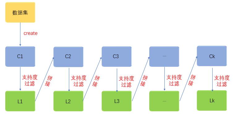
Apriori算法

　　发现频繁项集的过程如上图所示：

由数据集生成候选项集C1（1表示每个候选项仅有一个数据项）；再由C1通过支持度过滤，生成频繁项集L1（1表示每个频繁项仅有一个数据项）。
将L1的数据项两两拼接成C2。
从候选项集C2开始，通过支持度过滤生成L2。L2根据Apriori原理拼接成候选项集C3；C3通过支持度过滤生成L3……直到Lk中仅有一个或没有数据项为止。

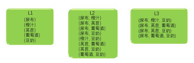
　　回到上面的杂货店例子，令最小支持度为0.4，结果如下图：

　　值得注意的是L3到C4这一步并没有得到候选项集，这是由于Apriori算法由两部分组成（在这里假定购买商品是有顺序的）。

连接：对K-1项集中的每个项集中的项排序，只有在前K-1项相同时才将这两项合并，形成候选K项集（因为必须形成K项集，所以只有在前K-1项相同，第K项不相同的情况下才合并。）
剪枝：对于候选K项集，要验证所有项集的所有K-1子集是否频繁（是否在K-1项集中），去掉不满足的项集，就形成了K项集。比如C4连接的｛尿布，莴苣，葡萄酒，豆奶｝的子集｛莴苣，葡萄酒，豆奶｝不存在于L3，因此要去掉。

实现Apriori代码

　　根据以上原理构造数据集扫描的Python代码，其伪代码大致如下：

对数据集中的每条交易记录tran
对每个候选项集can :
    检查一下can是否是tran的子集 :
    如果是，则增加can的计数值
对每个候选项集 :
如果其支持度不低于最小值，则保留该项集
返回所有频繁项集列表

　　建立辅助函数：

# 创建一个简单的测试数据集
def loadDataSet() :
    return [[1,3,4], [2,3,5], [1,2,3,5], [2,5]]

# 构建集合C1，C1是大小为1的所有候选项集的集合。
def createC1(dataSet) :
    # C1是空列表，用来存储所有不重复的项值。如果某个物品项没有在C1中出现，则将其添加到C1中。
    # 这里并不是简单地每个物品项，而是添加只包含该物品项的一个列表。Python不能创建只有一个整
    # 数的集合，因此这里实现必须使用列表
    C1 = []
    for transaction in dataSet :
        for item in transaction :
            if not [item] in C1 :
                C1.append([item])
    C1.sort()
    # frozenset是指被“冰冻”的集合，就是说它们是不可改变
    return list(map(frozenset,C1)) 

# D: 数据集
# Ck: 候选项集列表
# minSupport: 感兴趣集的最小支持度minSupport
# 该函数会返回一个包含支持度的字典以备后用
def scanD(D, Ck, minSupport) :
    ssCnt = {}
    for tid in D :
        for can in Ck :
            if can.issubset(tid) :
                if not can in ssCnt: ssCnt[can]=1
                else : ssCnt[can] += 1
    numItems = float(len(D))
    retList = []
    supportData = {}
    for key in ssCnt :
        # 计算所有项集的支持度
        support = ssCnt[key]/numItems
        if support >= minSupport :
            # 在列表的首部插入新的集合
            retList.insert(0, key)
        supportData[key] = support
    return retList, supportData

　　保存为apriori.py，运行效果如下：

>>> import apriori
# 导入数据集
>>> dataSet = apriori.loadDataSet()
>>> dataSet
[[1, 3, 4], [2, 3, 5], [1, 2, 3, 5], [2, 5]]
# 构建第一个候选项集集合C1
>>> C1 = apriori.createC1(dataSet)
>>> C1
[frozenset([1]), frozenset([2]), frozenset([3]), frozenset([4]), frozenset([5])]
# 构建集合表示的数据集D
>>> D = list(map(set, dataSet))
>>> D
[{1, 3, 4}, {2, 3, 5}, {1, 2, 3, 5}, {2, 5}]
# 去掉不满足最小支持度的项集，0.5为最小支持度
>>> L1, suppData0 = apriori.scanD(D, C1, 0.5)
# 下面四个项集构成了L1列表，该列表中每个单物品项集至少出现在50%以上的记录中
>>> L1
[frozenset([5]), frozenset([2]), frozenset([3]), frozenset([1])]

　　整个Apriori算法的伪代码如下：

当集合中项的个数大于0时
    构建一个k个项组成的候选项集的列表
    检查数据以确认每个项集都是频繁的
    保留频繁项集并构建k+1项组成的候选项集的列表

　　将如下算法代码加入apriori.py：

# 创建候选项集Ck
# Lk，频繁项集列表
# k，项集元素的个数
def aprioriGen(Lk, k) : # create Ck
    # 创建一个空列表
    retList = []
    # 计算Lk中的元素
    lenLk = len(Lk)
    for i in range(lenLk) :
        for j in range(i+1, lenLk) :
            # 当前k-2个项相同时，将两个集合合并
            L1 = list(Lk[i])[:k-2]
            L2 = list(Lk[j])[:k-2]
            L1.sort()
            L2.sort()
            if L1==L2 :
                # python中集合的并操作对应的操作符为|
                retList.append(Lk[i] | Lk[j])
    return retList

# dataSet，数据集
# minSupport，支持度
# 此函数会生成候选项集的列表
def apriori(dataSet, minSupport = 0.5) :
    C1 = createC1(dataSet)
    # map函数将set()映射到dataSet列表中的每一项
    D = list(map(set, dataSet))
    L1, supportData = scanD(D, C1, minSupport)
    # 将L1放入L列表中
    L = [L1]
    k = 2
    # while循环将L2, L3, L4, ... 放入L列表中，直到下一个大的项集为空
    while (len(L[k-2]) > 0) :
        # 调用aprioriGen()创建候选项集Ck
        Ck = aprioriGen(L[k-2], k)
        # 扫描数据集，从Ck得到Lk
        Lk, supK = scanD(D, Ck, minSupport)
        supportData.update(supK)
        L.append(Lk)
        k += 1
    return L, supportData

　　上面的k-2可能会令人困惑，接下来讨论其细节。当利用{0}、{1}、{2}构建{0,1}、{0,2}、{1,2}时，实际上是将单个项组合到一块。现在如果想利用{0,1}、{0,2}、{1,2}来创建三元素项集，应该怎么做？如果将每两个集合合并，就会得到{0,1,2}、{0,1,2}、{0,1,2}。也就是同样的结果集合会重复3次。接下来需要扫描三元素项集列表来得到非重复结果，我们要做的是确保遍历列表的次数最少。现在，如果比较集合{0,1}、{0,2}、{1,2}的第一个元素并只对第一个元素相同的集合求并操作，又会得到什么结果？{0,1,2}，而且只有一次操作，这样就不用遍历列表来寻找非重复值了。

　　保存后运行效果如下：

>>> L, supportData = apriori.apriori(dataSet)
>>> L
[[frozenset([5]), frozenset([2]), frozenset([3]), frozenset([1])], [frozenset([2
, 3]), frozenset([3, 5]), frozenset([2, 5]), frozenset([1, 3])], [frozenset([2,
3, 5])], []]
# L包含满足最小支持度为0.5的频率项集列表，下面看一下具体值：
>>> L[0]
[frozenset([5]), frozenset([2]), frozenset([3]), frozenset([1])]
>>> L[1]
[frozenset([2, 3]), frozenset([3, 5]), frozenset([2, 5]), frozenset([1, 3])]
>>> L[2]
[frozenset([2, 3, 5])]
>>> L[3]
[]
# 每个项集都是在函数apriori()中调用函数aprioriGen()来生成的。下面看一下aprioriGen()函数的工作流程：
>>> apriori.aprioriGen(L[0], 2)
[frozenset([2, 5]), frozenset([3, 5]), frozenset([1, 5]), frozenset([2, 3]), fro
zenset([1, 2]), frozenset([1, 3])]
# 这里的6个集合是候选项集Ck中的元素。其中4个集合在L[1]中，剩下2个集合被函数scanD()过滤掉。
# 下面再尝试70%的支持度：
>>> L,support = apriori.apriori(dataSet, minSupport=0.7)
>>> L
[[frozenset([5]), frozenset([2]), frozenset([3])], [frozenset([2, 5])], []]

从频繁项集中挖掘关联规则

　　关联分析的两个重要目标是发现频繁项集与关联规则。要找到关联规则，首先从一个频繁项集开始，集合中的元素是不重复的，但我们想知道基于这些元素能否获得其他内容。某个元素或者某个元素集合可能会推导出另一个元素。例如，一个频繁项集｛豆奶, 莴苣｝，可能有一条关联规则“豆奶→莴苣”，这意味着如果有人购买了豆奶，那么在统计上他购买莴苣的概率较大。但是这条反过来并不总是成立。换言之，即使“豆奶→莴苣”统计上显著，那么“莴苣→豆奶”也不一定成立。箭头的左边集合称作前件，箭头右边的集合称为后件。

　　上节我们给出了繁琐项集的量化定义，即它满足最小支持度要求。对于关联规则，我们也有类似量化方法，这种量化标准称为可信度。一条规则P→H的可信度定义为support(P | H) / support(P)。在前面我们已经计算了所有繁琐项集支持度，要想获得可信度，只需要再做一次除法运算。

　　从一个繁琐项集中可以产生多少条关联规则？下图给出了从项集{0,1,2,3}产生的所有关联规则。为了找到感兴趣的规则，我们先生成一个可能的规则列表，然后测试每条规则可信度。如果可信度不满足最小要求，则去掉该规则。

　　可以观察到，如果某条规则并不满足最小可信度要求，那么该规则的所有子集也不会满足最小可信度要求。具体而言，如果012→3是一条低可信度规则，则所有其它3为后件的规则都是低可信度。这需要从可信度的概念去理解，Confidence(012→3) = P(3|0,1,2), Confidence(01→23)=P(2,3|0,1)，P(3|0,1,2) >= P(2,3|0,1)。由此可以对关联规则做剪枝处理。

　　还是以之前的杂货店交易数据为例，我们发现了以下频繁项集：

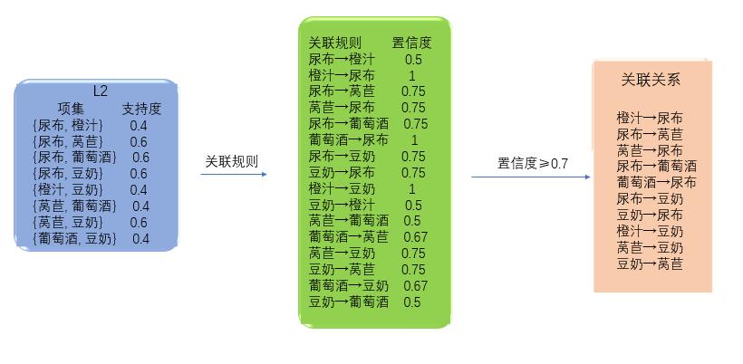
　　对于寻找关联规则来说，频繁1项集L1没有用处，因为L1中的每个集合仅有一个数据项，至少有两个数据项才能生成A→B这样的关联规则。取置信度为0.7，最终从L2发掘出10条关联规则：

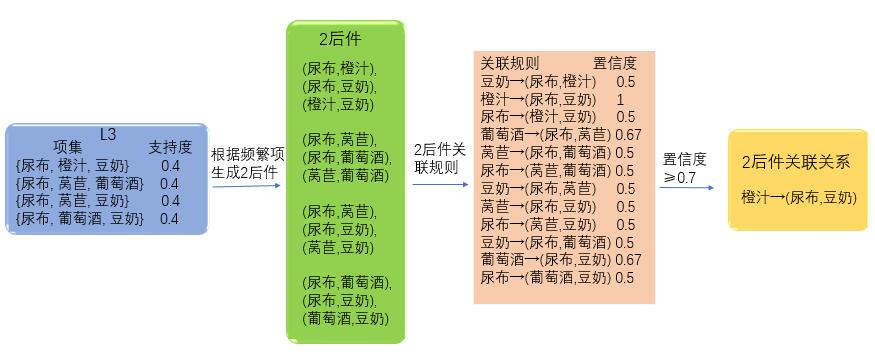
　　接下来是L3：

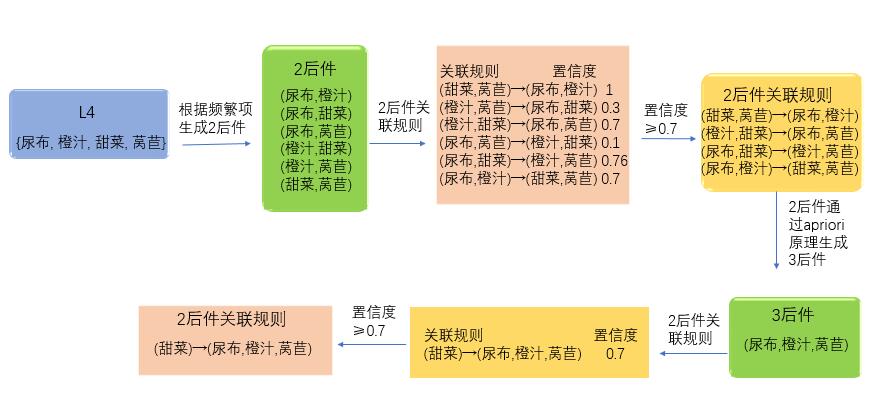
　　假设有一个L4项集（文中的数据不能生成L4），其挖掘过程如下：

　　利用此性质来减少测试的规则数目，可以先从一个频繁项集开始，接着创建一个规则列表，其中规则右部只包含一个元素，然后对这些规则测试。接下来合并所有剩余规则来创建一个新的规则列表，其中右部包含两个元素。这种方法称为分级法。打开apriori.py，加入如下代码：

# 关联规则生成函数，此函数调用其他两个函数rulesFromConseq、calcConf
# L: 频繁项集列表
# supportData: 包含那些频繁项集支持数据的字典
# minConf: 最小可信度阈值，默认是0.7
# 函数最后要生成一个包含可信度的规则列表，后面可以基于可信度对它们进行排序
# 这些规则存放在bigRuleList中。
def generateRules(L, supportData, minConf=0.7) :
    bigRuleList = []
    # 遍历L中的每一个频繁项集并对每个频繁项集创建只包含单个元素集合的列表H1，
    # 因为无法从单元素项集中构建关联规则，所以要从包含两个或者更多元素的项集开始规则构建过程。

    # 只获取有两个或更多元素的集合
    for i in range(1, len(L)) :
        for freqSet in L[i] :
            H1 = [frozenset([item]) for item in freqSet]
            if i > 1 :
                # 如果频繁项集的元素数目超过2，那么会考虑对它做进一步的合并，合并通过
                # rulesFromConseq来完成
                rulesFromConseq(freqSet, H1, supportData, bigRuleList, minConf)
            else :
                # 如果项集中只有两个元素，那么需要使用calcConf()来计算可信度值
                calcConf(freqSet, H1, supportData, bigRuleList, minConf)
    return bigRuleList

# 对规则进行评估
# 目标是计算规则的可信度以及找到满足最小可信度要求的规则
# 函数会返回一个满足最小可信度要求的规则列表，空列表prunedH保存这些规则
def calcConf(freqSet, H, supportData, brl, minConf=0.7) :
    prunedH = []
    # 遍历H中的所有项集并计算它们的可信度值
    for conseq in H :
        # 可信度计算时使用supportData中的支持度数据
        conf = supportData[freqSet] / supportData[freqSet - conseq]
        # 规则满足最小可信度值，将这些规则输出到屏幕显示
        if conf >= minConf :
            print(freqSet-conseq, '-->', conseq, 'conf:', conf)
            brl.append((freqSet-conseq, conseq, conf))
            prunedH.append(conseq)
    return prunedH

# 用于生成候选规则集合，从最初的项集中生成更多的关联规则
# freqSet: 频繁项集
# H: 可以出现在规则右部的元素列表
def rulesFromConseq(freqSet, H, supportData, brl, minConf=0.7) :
    # H中频繁项集大小m
    m = len(H[0])
    # 查看该频繁项集是否大到可以移除大小为m的子集
    if (len(freqSet) > (m+1)) :
        # 生成H中元素的无重复组合，结果存储在Hmp1，这也是下一次迭代的H列表
        Hmp1 = aprioriGen(H, m+1)
        # Hmp1包含所有可能的规则，利用calcConf()来测试它们的可信度以确定是否满足要求
        Hmp1 = calcConf(freqSet, Hmp1, supportData, brl, minConf)
        # 如果不止一条规则满足要求，那么使用Hmp1迭代调用函数rulesFromConseq
        if (len(Hmp1) > 1) :
            rulesFromConseq(freqSet, Hmp1, supportData, brl, minConf)

　　检验运行效果：

>>> import apriori
>>> dataSet = apriori.loadDataSet()
>>> dataSet
[[1, 3, 4], [2, 3, 5], [1, 2, 3, 5], [2, 5]]
# 生成一个最小支持度为0.5的频繁项集的集合
>>> L, supportData = apriori.apriori(dataSet, minSupport=0.5)
>>> rules = apriori.generateRules(L, supportData, minConf=0.7)
frozenset([5]) --> frozenset([2]) conf: 1.0
frozenset([2]) --> frozenset([5]) conf: 1.0
frozenset([1]) --> frozenset([3]) conf: 1.0
>>> rules
[(frozenset([5]), frozenset([2]), 1.0), (frozenset([2]), frozenset([5]), 1.0), (
frozenset([1]), frozenset([3]), 1.0)]
# 得到了3条规则：{5}→{2}、{2}→{5}、{1}→{3}，可见包含2和5的规则可以互换前后件，包含1和3的不行
# 接下来降低可信度阈值，可以得到结果如下
>>> rules = apriori.generateRules(L, supportData, minConf=0.5)
frozenset([3]) --> frozenset([2]) conf: 0.666666666667
frozenset([2]) --> frozenset([3]) conf: 0.666666666667
frozenset([5]) --> frozenset([3]) conf: 0.666666666667
frozenset([3]) --> frozenset([5]) conf: 0.666666666667
frozenset([5]) --> frozenset([2]) conf: 1.0
frozenset([2]) --> frozenset([5]) conf: 1.0
frozenset([3]) --> frozenset([1]) conf: 0.666666666667
frozenset([1]) --> frozenset([3]) conf: 1.0
frozenset([5]) --> frozenset([2, 3]) conf: 0.666666666667
frozenset([3]) --> frozenset([2, 5]) conf: 0.666666666667
frozenset([2]) --> frozenset([3, 5]) conf: 0.666666666667
>>> rules
[(frozenset({3}), frozenset({2}), 0.6666666666666666), (frozenset({2}), frozenset({3}), 0.6666666666666666), (frozenset({5}), frozenset({3}), 0.6666666666666666), (frozenset({3}), frozenset({5}), 0.6666666666666666), (frozenset({5}), frozenset({2}), 1.0), (frozenset({2}), frozenset({5}), 1.0), (frozenset({3}), frozenset({1}), 0.6666666666666666), (frozenset({1}), frozenset({3}), 1.0), (frozenset({5}), frozenset({2, 3}), 0.6666666666666666), (frozenset({3}), frozenset({2, 5}), 0.6666666666666666), (frozenset({2}), frozenset({3, 5}), 0.6666666666666666)]
# 一旦降低可信度阈值，就可以获得更多的规则

Apriori应用

　　之前我们在小数据上应用了apriori算法，接下来要在更大的真实数据集上测试效果。那么可以使用什么样的数据呢？比如：购物篮分析，搜索引擎的查询词，国会投票，毒蘑菇的相似特征提取等；

示例：发现毒蘑菇的相似特征

　　从此处下载mushroom.dat，其前几行如下：

1 3 9 13 23 25 34 36 38 40 52 54 59 63 67 76 85 86 90 93 98 107 113 
2 3 9 14 23 26 34 36 39 40 52 55 59 63 67 76 85 86 90 93 99 108 114 
2 4 9 15 23 27 34 36 39 41 52 55 59 63 67 76 85 86 90 93 99 108 115 
1 3 10 15 23 25 34 36 38 41 52 54 59 63 67 76 85 86 90 93 98 107 113 
2 3 9 16 24 28 34 37 39 40 53 54 59 63 67 76 85 86 90 94 99 109 114 
2 3 10 14 23 26 34 36 39 41 52 55 59 63 67 76 85 86 90 93 98 108 114 
2 4 9 15 23 26 34 36 39 42 52 55 59 63 67 76 85 86 90 93 98 108 115

　　第一个特征表示有毒或者可食用，有毒为2，无毒为1。下一个特征是蘑菇伞的形状，有六种可能的值，分别用整数3-8来表示。

　　为了找到毒蘑菇中存在的公共特征，可以运行Apriori算法来寻找包含特征值为2的频繁项集。

>>> import apriori
>>> mushDatSet = [line.split() for line in open('mushroom.dat').readlines()]
# 在数据集上运行Apriori算法
>>> L, suppData = apriori.apriori(mushDatSet, minSupport=0.3)
# 在结果中可以搜索包含有独特征2的频繁项集：
>>> for item in L[1] :
...		if item.intersection('2'): print(item)
...
frozenset({'28', '2'})
frozenset({'2', '53'})
frozenset({'2', '23'})
frozenset({'2', '34'})
frozenset({'2', '36'})
frozenset({'59', '2'})
frozenset({'63', '2'})
frozenset({'67', '2'})
frozenset({'2', '76'})
frozenset({'2', '85'})
frozenset({'2', '86'})
frozenset({'2', '90'})
frozenset({'93', '2'})
frozenset({'2', '39'})
# 对更大项集来重复上述过程
>>> for item in L[3] :
...     if item.intersection('2') : print(item)
...
frozenset({'2', '28', '59', '34'})
frozenset({'2', '28', '59', '85'})
frozenset({'2', '86', '28', '59'})
frozenset({'2', '28', '59', '90'})
frozenset({'2', '28', '59', '39'})
frozenset({'63', '2', '28', '39'})
frozenset({'63', '2', '28', '34'})
frozenset({'63', '2', '28', '59'})
frozenset({'63', '2', '28', '85'})
frozenset({'63', '2', '86', '28'})
frozenset({'2', '28', '85', '34'})
frozenset({'2', '86', '28', '34'})
frozenset({'2', '86', '28', '85'})
frozenset({'34', '2', '28', '90'})
frozenset({'2', '28', '85', '90'})
frozenset({'2', '86', '28', '90'})
frozenset({'2', '28', '34', '39'})
frozenset({'2', '28', '85', '39'})
frozenset({'2', '86', '28', '39'})
frozenset({'2', '28', '90', '39'})
frozenset({'34', '2', '28', '53'})
frozenset({'2', '28', '85', '53'})
frozenset({'2', '86', '28', '53'})
frozenset({'90', '2', '28', '53'})
frozenset({'2', '28', '53', '39'})
......

　　接下来你需要观察这些特征，以便知道蘑菇的各个方面，如果看到其中任何一个特征，那么这些蘑菇就很有可能有毒。

小结

　　关联特征是用于发现大数据集元素间有趣关系的一个工具集，可以采用两种方法来量化这些有趣关系。第一种方法是使用频繁项集，它会给出经常在一起出现的元素项。第二种方式是关联规则，每条关联规则意味着元素之前的“如果……那么”关系。

　　发现元素间不同的组合是个非常耗时的任务，不可避免需要大量昂贵的计算资源，这就需要一些更智能的方法在合适的时间范围内找到频繁项集。其中一个方法是Apriori算法，它使用Apriori原理减少在数据库上进行检查的集合的数目。Apriori原理是说如果一个元素项是不频繁的，那么那些包含该元素的超集也是不频繁的。Apriori算法从单元项集开始，通过组合满足最小支持度要求的项集来形成更大的集合。支持度用来度量一个集合在原始数据中出现的频率。

　　关联分析可以用在许多不同物品上。商店中的商品以及网站的访问页面是其中比较常见的例子。关联分析也曾用于查看选举人及法官的投票历史。

　　缺点是每次增加频繁项集的大小，Apriori算法都会重新扫描整个数据集，当数据集很大时，这会显著降低频繁项集发现的速度。

参考资料：《机器学习实战》、《数据挖掘导论》

# Apriori, Association Analysis, Data Mining, Machine Learning, Python