记录一下学习分子动力学(Gromacs)的流程,希望给后人提供一点帮助。
工作环境 Gromacs 需要在Linux下安装,再次不赘述如何安装ubuntu双系统/子系统的方法,可以自行搜索。
1
2
3
4
5
conda create --name gmx python=3.7.3 conda activate gmx conda install gromacs
1
2
3
4
5
conda config --add channels http://mirrors.tuna.tsinghua.edu.cn/anaconda/pkgs/free/ conda config --add channels http://mirrors.tuna.tsinghua.edu.cn/anaconda/pkgs/main/ conda config --set show_channel_urls yes conda config --add channels http://mirrors.tuna.tsinghua.edu.cn/anaconda/cloud/conda-forge/ conda config --add channels http://mirrors.tuna.tsinghua.edu.cn/anaconda/cloud/bioconda/
1 conda install networkx=2.3
avogadro 用于给配体加氢操作,访问avogadro 下载安装。
CHARMM36 访问网站 ,下载CHARMM36力场,访问网站 ,下载对应cgenff_charmm2gmx脚本,解压至工作目录。
sort_mol2_bonds.pl 处理分子的脚本文件,访问此处 下载,本项目选择的是cgenff_charmm2gmx_py3_nx2.py,解压至工作目录。
Qtgrace 适合快速预览可视化,点此 下载。
基本常识 首先需要稍微了解一下各文件含义和表示方法,当然跳过直接做应该也行。
mol2 以下为一个分子的mol2文件,显示如下,我将关键信息以注释形式标记:
1
2
3
4
5
6
7
8
9
10
11
12
13
14
15
16
17
18
19
20
@<TRIPOS>MOLECULE UNL1 # 分子名 75 79 0 0 0 # 第一个代表有75个原子 SMALL GASTEIGER # GASTEIGER电荷,代表一种电荷形式,由力场产生 # 第一列代表原子序号 # 第二列代表元素 # 中间三列代表XYZ,即坐标 # 第六列代表原子类型,如阿尔法碳原子 # 第七列代表分子序数 # 第八列为分子名称简写 # 最后一列原子电荷 @<TRIPOS>ATOM 1 N 12.7250 10.5600 -29.9030 N.3 1 UNL1 -0.2511 2 N 11.8620 9.5520 -29.5930 N.3 1 UNL1 -0.2289 3 N 18.2190 12.7890 -33.9180 N.3 1 UNL1 -0.2750 4 N 20.6040 13.9660 -34.9820 N.3 1 UNL1 -0.2751 5 C 18.2320 11.3310 -31.1210 C.3 1 UNL1 0.1074 6 C 18.0730 11.2020 -29.7430 C.3 1 UNL1 -0.0211
pdb 以下为一个分子的mol2文件,显示如下,我将关键信息以注释形式标记:
1
2
3
4
5
6
7
8
9
10
11
12
13
14
15
16
17
18
19
20
21
# 第一列代表原子 # 第二列代表原子序号 # 第三列代表原子类型,比如CA是阿尔法碳原子 # 第四列代表氨基酸缩写 # 第五列代表蛋白质的链 # 第六列代表氨基酸残基编号,如3就是3号残基 # 第七到九列代表代表XYZ # 第十列代表占位比,1.00即代表该原子在该位置出现概率为100% # 第十一列代表温度因子,原子热振动程度 # 最后一列为元素 # 如果计算电荷,还能多一列电荷信息 ATOM 34 N ASP A 3 27.619 20.810 -7.568 1.00 0.49 N ATOM 35 CA ASP A 3 28.326 21.638 -8.592 1.00 0.49 C ATOM 36 C ASP A 3 29.110 20.808 -9.598 1.00 0.49 C ATOM 37 O ASP A 3 29.501 19.679 -9.308 1.00 0.49 O ATOM 38 CB ASP A 3 29.198 22.696 -7.862 1.00 0.49 C ATOM 39 CG ASP A 3 28.341 23.607 -6.998 1.00 0.49 C ATOM 40 OD1 ASP A 3 27.122 23.300 -6.909 1.00 0.49 O ATOM 41 OD2 ASP A 3 28.899 24.541 -6.394 1.00 0.49 O1- ATOM 42 N VAL A 4 29.299 21.335 -10.822 1.00 0.74 N
操作步骤 生成拓扑
将对接复合物的pdb文件以文本格式打开,复合物前面为小分子,剪切出来新建为mol.pdb文件,剩下部分保存为pro.pdb文件;
使用avogadro打开mol.pdb文件,构建—氢原子—添加氢原子,文件—输出为mol.mol2文件
1 2 3 4 cd dygmx pdb2gmx -f pro.pdb -o protein_processed.gro -ignh perl sort_mol2_bonds.pl mol.mol2 mol_fix.mol2
文本编辑器打开mol2文件,把@MOLECULE下的星号替换成正确残基名,为了方便演示,这里我暂定义为resi。
访问CGenFF ,需用教育网邮箱注册,将上面fixed的mol2文件上传,转换为str文件下载。
1
2
python cgenff_charmm2gmx_py3_nx2.py resi mol_fix.mol2 mol_fix.str charmm36-jul2022.ff gmx editconf -f resi_ini.pdb -o resi.gro
此时已经生成了两个gro文件,新建文本文档,命名为complex.gro,首先将蛋白质的gro文件全部内容复制过去,再将小分子第三行到倒数第二行复制,插入到先前蛋白质的最后一行以前。下面为为示例数据:
1
2
3
4
163ASN C 1691 0.621 -0.740 -0.126 163ASN O1 1692 0.624 -0.616 -0.140 163ASN O2 1693 0.683 -0.703 -0.011 5.99500 5.19182 9.66100 0.00000 0.00000 -2.99750 0.00000 0.00000 0.00000
1
2
3
4
5
6
7
8
9
10
11
12
13
14
15
16
17
18
19
20
21
22
23
24
25
26
27
28
163ASN C 1691 0.621 -0.740 -0.126 163ASN O1 1692 0.624 -0.616 -0.140 163ASN O2 1693 0.683 -0.703 -0.011 1JZ4 C4 1 2.429 -2.412 -0.007 1JZ4C7 2 2.155 -2.721 -0.411 1JZ4C8 3 2.207 -2.675 -0.533 1JZ4 C9 4 2.267 -2.551 -0.545 1JZ4 C10 5 2.277 -2.473 -0.430 1JZ4 C11 6 2.169 -2.646 -0.295 1JZ4 C12 7 2.229 -2.519 -0.308 1JZ4 C13 8 2.246 -2.441 -0.181 1JZ4 C14 9 2.392 -2.470 -0.139 1JZ4 OAB 10 2.341 -2.354 -0.434 1JZ4 H1 11 2.531 -2.436 0.015 1JZ4 H2 12 2.366 -2.453 0.069 1JZ4 H3 13 2.417 -2.306 -0.010 1JZ4 H4 14 2.107 -2.812 -0.407 1JZ4 H5 15 2.199 -2.735 -0.617 1JZ4H6 16 2.304 -2.518 -0.635 1JZ4H7 17 2.137 -2.681 -0.204 1JZ4 H8 18 2.178 -2.476 -0.106 1JZ4 H9 19 2.227 -2.337 -0.193 1JZ4 H10 20 2.458 -2.429 -0.214 1JZ4 H11 21 2.402 -2.577 -0.131 1JZ4 H12 22 2.374 -2.321 -0.516 5.99500 5.19182 9.66100 0.00000 0.00000 -2.99750 0.00000 0.00000 0.00000
此时复合物文件的原子数为2个文件之和,因此需要在第2行把2个文件原子数相加并保存。
再打开topol.top文件,在[ moleculetype ] 以上添加如下信息:
1
2
; Include ligand parameters
1
2
; Include ligand topology
再拉到最后面,[ molecules ] 项,在Protein_chain_A 下添加:
定义盒子
1
2
gmx editconf -f complex.gro -o newbox.gro -bt dodecahedron -d 1.0 gmx solvate -cp newbox.gro -cs spc216.gro -p topol.top -o solv.gro
添加离子
构建完盒子后,现在得到了一个带电蛋白质的溶剂化系统(如果打开topol.top,看到[ atoms ] 项目中会存在类似于qtot 6字段),因此需要在系统中添加离子。
新建ions.mdp文件,将下列代码粘贴进去并保存:
1
2
3
4
5
6
7
8
9
10
11
12
13
14
15
16
17
18
; LINES STARTING WITH ';' ARE COMMENTS title = Minimization ; Title of run ; Parameters describing what to do , when to stop and what to save integrator = steep ; Algorithm (steep = steepest descent minimization) emtol = 1000.0 ; Stop minimization when the maximum force < 10.0 kJ/mol emstep = 0.01 ; Energy step size nsteps = 50000 ; Maximum number of (minimization) steps to perform ; Parameters describing how to find the neighbors of each atom and how to calculate the interactions nstlist = 1 ; Frequency to update the neighbor list and long range forces cutoff-scheme = Verlet ns_type = grid ; Method to determine neighbor list (simple, grid) rlist = 1.0 ; Cut-off for making neighbor list (short range forces) coulombtype = cutoff ; Treatment of long range electrostatic interactions rcoulomb = 1.0 ; long range electrostatic cut-off rvdw = 1.0 ; long range Van der Waals cut-off pbc = xyz ; Periodic Boundary Conditions
1 2 3 gmx grompp -f ions.mdp -c solv.gro -p topol.top -o ions.tpr gmx genion -s ions.tpr -o solv_ions.gro -p topol.top -pname NA -nname CL -neutral
此时如果访问topol.top拖到最下面应该可以看到添加了离子。
能量最小化
动力学模拟需要把让系统处于能量最小值,先新建em.mdp文件,粘贴以下内容并保存:
1
2
3
4
5
6
7
8
9
10
11
12
13
14
15
16
17
18
19
20
21
22
; LINES STARTING WITH ';' ARE COMMENTS title = Minimization ; Title of run ; Parameters describing what to do , when to stop and what to save integrator = steep ; Algorithm (steep = steepest descent minimization) emtol = 1000.0 ; Stop minimization when the maximum force < 10.0 kJ/mol emstep = 0.01 ; Energy step size nsteps = 50000 ; Maximum number of (minimization) steps to perform ; Parameters describing how to find the neighbors of each atom and how to calculate the interactions nstlist = 1 ; Frequency to update the neighbor list and long range forces cutoff-scheme = Verlet ns_type = grid ; Method to determine neighbor list (simple, grid) rlist = 1.2 ; Cut-off for making neighbor list (short range forces) coulombtype = PME ; Treatment of long range electrostatic interactions rcoulomb = 1.2 ; long range electrostatic cut-off vdwtype = cutoff vdw-modifier = force-switch rvdw-switch = 1.0 rvdw = 1.2 ; long range Van der Waals cut-off pbc = xyz ; Periodic Boundary Conditions DispCorr = no
如果后续报错,可以换成这个em.mdp,原理可能是steep算法问题,替换掉不会过于激进,也有可能是define = -DFLEXIBLE这段改变了什么条件,且不去深究了。
1
2
3
4
5
6
7
8
9
10
11
12
13
14
15
16
17
18
19
20
21
22
23
24
25
26
27
28
29
30
31
32
33
34
; VARIOUS PREPROCESSING OPTIONS = title = include = define = -DFLEXIBLE ; RUN CONTROL PARAMETERS = integrator = cg ; start time and timestep in ps = tinit = 0 dt = 0.001 nsteps = 100 ; ENERGY MINIMIZATION OPTIONS = emtol = 0.00001 emstep = 0.001 nstcgsteep = 1000 ; OUTPUT CONTROL OPTIONS ; Output frequency for coords (x), velocities (v) and forces (f) nstxout = 0 nstvout = 0 nstfout = 0 ; Output frequency for energies to log file and energy file nstlog = 0 nstcalcenergy = -1 nstenergy = 0 ; Output frequency and precision for .xtc file nstxtcout = 0 lincs_order = 8 rcoulomb = 0.9 rvdw = 0.9 rlist = 0.9
1
2
gmx grompp -f em.mdp -c solv_ions.gro -p topol.top -o em.tpr gmx mdrun -v -deffnm em
平衡 约束配体
1
2
3
4
gmx make_ndx -f resi.gro -o index_resi.ndx ... > 0 & ! a H* > q
1 2 gmx genrestr -f resi.gro -n index_resi.ndx -o posre_resi.itp -fc 1000 1000 1000
然后需要处理topol.top文件,打开拉到底部区域,定位到; Include water topology处,在前面插入并保存:
1
2
3
4
; Ligand position restraints
恒温器
1
2
3
4
5
gmx make_ndx -f em.gro -o index.ndx ... > 1 | 13 > q
再做NVT平衡,新建nvt.mdp,粘贴以下内容并保存,但是注意里面有个字段要修改! 找到tc-grps,把后面的Protein_JZ4改成上一部合并的蛋白质残基索引!
1
2
3
4
5
6
7
8
9
10
11
12
13
14
15
16
17
18
19
20
21
22
23
24
25
26
27
28
29
30
31
32
33
34
35
36
37
38
39
40
41
42
43
44
45
title = Protein-ligand complex NVT equilibration define = -DPOSRES ; position restrain the protein and ligand ; Run parameters integrator = md ; leap-frog integrator nsteps = 50000 ; 2 * 50000 = 100 ps dt = 0.002 ; 2 fs ; Output control nstenergy = 500 ; save energies every 1.0 ps nstlog = 500 ; update log file every 1.0 ps nstxout-compressed = 500 ; save coordinates every 1.0 ps ; Bond parameters continuation = no ; first dynamics run constraint_algorithm = lincs ; holonomic constraints constraints = h-bonds ; bonds to H are constrained lincs_iter = 1 ; accuracy of LINCS lincs_order = 4 ; also related to accuracy ; Neighbor searching and vdW cutoff-scheme = Verlet ns_type = grid ; search neighboring grid cells nstlist = 20 ; largely irrelevant with Verlet rlist = 1.2 vdwtype = cutoff vdw-modifier = force-switch rvdw-switch = 1.0 rvdw = 1.2 ; short-range van der Waals cutoff (in nm) ; Electrostatics coulombtype = PME ; Particle Mesh Ewald for long-range electrostatics rcoulomb = 1.2 ; short-range electrostatic cutoff (in nm) pme_order = 4 ; cubic interpolation fourierspacing = 0.16 ; grid spacing for FFT ; Temperature coupling tcoupl = V-rescale ; modified Berendsen thermostat tc-grps = Protein_JZ4 Water_and_ions ; two coupling groups - more accurate tau_t = 0.1 0.1 ; time constant, in ps ref_t = 300 300 ; reference temperature, one for each group, in K ; Pressure coupling pcoupl = no ; no pressure coupling in NVT ; Periodic boundary conditions pbc = xyz ; 3-D PBC ; Dispersion correction is not used for proteins with the C36 additive FF DispCorr = no ; Velocity generation gen_vel = yes ; assign velocities from Maxwell distribution gen_temp = 300 ; temperature for Maxwell distribution gen_seed = -1 ; generate a random seed
1
2
3
gmx grompp -f nvt.mdp -c em.gro -r em.gro -p topol.top -n index.ndx -o nvt.tpr gmx mdrun -v -deffnm nvt
然后做再做NPT平衡,新建npt.mdp,粘贴以下内容并保存,一样要改tc-grps!
1
2
3
4
5
6
7
8
9
10
11
12
13
14
15
16
17
18
19
20
21
22
23
24
25
26
27
28
29
30
31
32
33
34
35
36
37
38
39
40
41
42
43
44
45
46
47
48
title = Protein-ligand complex NPT equilibration define = -DPOSRES ; position restrain the protein and ligand ; Run parameters integrator = md ; leap-frog integrator nsteps = 50000 ; 2 * 50000 = 100 ps dt = 0.002 ; 2 fs ; Output control nstenergy = 500 ; save energies every 1.0 ps nstlog = 500 ; update log file every 1.0 ps nstxout-compressed = 500 ; save coordinates every 1.0 ps ; Bond parameters continuation = yes ; continuing from NVT constraint_algorithm = lincs ; holonomic constraints constraints = h-bonds ; bonds to H are constrained lincs_iter = 1 ; accuracy of LINCS lincs_order = 4 ; also related to accuracy ; Neighbor searching and vdW cutoff-scheme = Verlet ns_type = grid ; search neighboring grid cells nstlist = 20 ; largely irrelevant with Verlet rlist = 1.2 vdwtype = cutoff vdw-modifier = force-switch rvdw-switch = 1.0 rvdw = 1.2 ; short-range van der Waals cutoff (in nm) ; Electrostatics coulombtype = PME ; Particle Mesh Ewald for long-range electrostatics rcoulomb = 1.2 pme_order = 4 ; cubic interpolation fourierspacing = 0.16 ; grid spacing for FFT ; Temperature coupling tcoupl = V-rescale ; modified Berendsen thermostat tc-grps = Protein_JZ4 Water_and_ions ; two coupling groups - more accurate tau_t = 0.1 0.1 ; time constant, in ps ref_t = 300 300 ; reference temperature, one for each group, in K ; Pressure coupling pcoupl = Berendsen ; pressure coupling is on for NPT pcoupltype = isotropic ; uniform scaling of box vectors tau_p = 2.0 ; time constant, in ps ref_p = 1.0 ; reference pressure, in bar compressibility = 4.5e-5 ; isothermal compressibility of water, bar^-1 refcoord_scaling = com ; Periodic boundary conditions pbc = xyz ; 3-D PBC ; Dispersion correction is not used for proteins with the C36 additive FF DispCorr = no ; Velocity generation gen_vel = no ; velocity generation off after NVT
1
2
3
gmx grompp -f npt.mdp -c nvt.gro -t nvt.cpt -r nvt.gro -p topol.top -n index.ndx -o npt.tpr gmx mdrun -v -deffnm npt
模拟
新建md.mdp文件,粘贴以下内容并保存,同样记得修改!
1
2
3
4
5
6
7
8
9
10
11
12
13
14
15
16
17
18
19
20
21
22
23
24
25
26
27
28
29
30
31
32
33
34
35
36
37
38
39
40
41
42
43
44
45
46
title = Protein-ligand complex MD simulation ; Run parameters integrator = md ; leap-frog integrator nsteps = 5000000 ; 2 * 5000000 = 10000 ps (10 ns) dt = 0.002 ; 2 fs ; Output control nstenergy = 5000 ; save energies every 10.0 ps nstlog = 5000 ; update log file every 10.0 ps nstxout-compressed = 5000 ; save coordinates every 10.0 ps ; Bond parameters continuation = yes ; continuing from NPT constraint_algorithm = lincs ; holonomic constraints constraints = h-bonds ; bonds to H are constrained lincs_iter = 1 ; accuracy of LINCS lincs_order = 4 ; also related to accuracy ; Neighbor searching and vdW cutoff-scheme = Verlet ns_type = grid ; search neighboring grid cells nstlist = 20 ; largely irrelevant with Verlet rlist = 1.2 vdwtype = cutoff vdw-modifier = force-switch rvdw-switch = 1.0 rvdw = 1.2 ; short-range van der Waals cutoff (in nm) ; Electrostatics coulombtype = PME ; Particle Mesh Ewald for long-range electrostatics rcoulomb = 1.2 pme_order = 4 ; cubic interpolation fourierspacing = 0.16 ; grid spacing for FFT ; Temperature coupling tcoupl = V-rescale ; modified Berendsen thermostat tc-grps = Protein_resi Water_and_ions ; two coupling groups - more accurate tau_t = 0.1 0.1 ; time constant, in ps ref_t = 300 300 ; reference temperature, one for each group, in K ; Pressure coupling pcoupl = Parrinello-Rahman ; pressure coupling is on for NPT pcoupltype = isotropic ; uniform scaling of box vectors tau_p = 2.0 ; time constant, in ps ref_p = 1.0 ; reference pressure, in bar compressibility = 4.5e-5 ; isothermal compressibility of water, bar^-1 ; Periodic boundary conditions pbc = xyz ; 3-D PBC ; Dispersion correction is not used for proteins with the C36 additive FF DispCorr = no ; Velocity generation gen_vel = no ; continuing from NPT equilibration
1
2
3
gmx grompp -f md.mdp -c npt.gro -t npt.cpt -p topol.top -n index.ndx -o md_0_10.tpr gmx mdrun -deffnm md_0_10
分析 直接运行代码吧:
1 2 3 4 5 6 7 8 9 10 11 12 13 14 15 16 17 18 19 20 21 22 23 24 25 work_path=$1 mol_name=$2 mol_root="$work_path /****/$mol_name " md_trr="$mol_root /md.trr" md_xtc="$mol_root /md.xtc" md_edr="$mol_root /md.edr" md_tpr="$mol_root /md.tpr" gmx trjconv -f $md_trr -o $md_xtc && \ printf "15\n" | gmx energy -f $md_edr -o "$mol_root /${mol_name} _energy.xvg" && \printf "1\n1\n" | gmx rms -f $md_xtc -s $md_tpr -o "$mol_root /${mol_name} _rmsd_protein.xvg" && \printf "4\n4\n" | gmx rms -f $md_xtc -s $md_tpr -o "$mol_root /${mol_name} _rmsd_backbone.xvg" && \printf "1\n13\n" | gmx rms -f $md_xtc -s $md_tpr -o "$mol_root /${mol_name} _rmsd_lig.xvg" && \printf "13\n13\n" | gmx rms -f $md_xtc -s $md_tpr -o "$mol_root /${mol_name} _rmsd_lig_lig.xvg" && \printf "1\n13\n" | gmx hbond -f $md_xtc -s $md_tpr -num "$mol_root /${mol_name} _hbnum.xvg"
xvg可以直接用Qtgrace可视化,也可以自己用matplotlib绘图。
一键式脚本 这里 有@kotori-y编写的一键MD脚本。
参考链接 Gromacs Tutorials :官方教程,非常细致,现存所有所有教程都是对官方教程的汉化。
速通版本-gromacs分子动力学模拟教程 :相当于上个教程视频化。
详细版本-用conda安装gromacs
中医药方向怎么发SCI?分子对接OUT了,快来学分子动力学模拟! :其中有段写作可参考的话术。
MDAnalysis
……